Polar Equations and the "n-leaf rose"
by
Stacy Musgrave
Let's warm up by looking at polar equations of the form
. We first look at some examples.
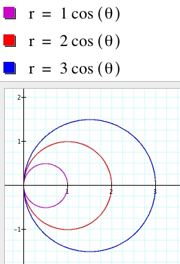
Let's fix k and change b:
So it appears that letting theta range from 0 to 2pi, we get circles of radius b.
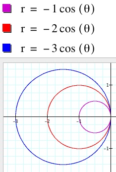
What happens if we make b negative? As one might expect based on the definition of parametric equations, changing the radius to it's negative will alter the circle. In this scenario, it appears like a reflection across the y-axis in the xy-plane. In reality, what's happening is that the original polar coordinate (theta, r) is being transformed to (theta, -r), which corresponds to a reflection through the origin of the original point. Reflecting the original three circles through the origin gives us the three new circles drawn with the same orientation. (If we were to trace the drawing of the original circles, we start at the the polar coordinate (0,b) and trace counterclockwise until we make full circle. So the picture we get after multiplying by -1 starts with polar coordinates (0, -b) and still goes counterclockwise until it makes a full circle.)
In either case, my main observation is that r can only be as large as the absolute value of b. So our picture will not venture beyond the scope of the circle centered at the origin with radius b.
Let's see if this holds even when we change the value of k. Again, we start by looking at examples, letting k take on various values:
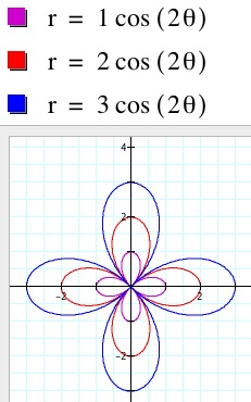
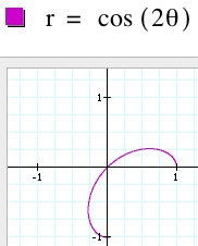
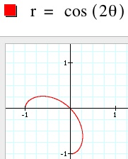
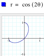
For k = 2:
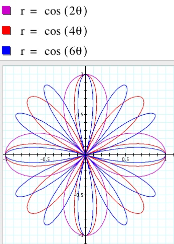
So we see even after changing the k value, the graph never reaches beyond the circle centered at the origin of radius b. However, we note an interesting change in the shape of our graph. Rather than forming a circle, we get a 4-leaf flower.
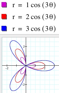
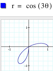
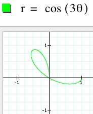
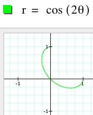
Check out k = 3:
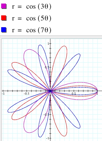
Again, the original claim seems to hold, as the images drawn are all contained in their respective circles of radius b centered at the origin. But again, an interesting development thanks to changing k to 3 is that we get a 3-leaf flower.
Claim: For a polar equation of the form
Proof: The proof is actually quite obvious. The k inside the parenthesis does not affect the range of the cosine function, which ranges between -1 and 1. So multiplying by b gives the range for r between -b and b. Since a negative r value corresponds to a vector of length b, the graph of our function will always lie inside (or on) the circle x2 + y2 = b2.
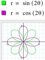
Point of Exploration: The last graph peaked my interest. If k= 2 led to a 4-leaf flower, should it not seem like a reasonable guess that k=3 would lead to a 6-leaf flower? Is it always true that for k even, we get a 2k-leaf flower and for n odd, we get a k-leaf flower?
Checking out some more graphs, letting b = 1 for convenience, we observe the following:
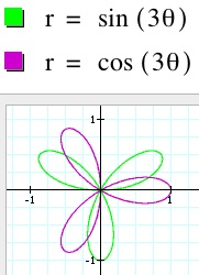
It seems that my original conjecture is correct. For even values of k, we get 2k-leaf flowers and for odd values of k, we get k-leaf flowers. So now we ask ourselves the most natural question: Why does this happen?
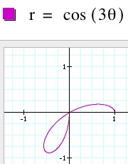
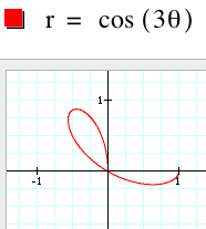
It may be instructive to take an odd graph step by step: For cos(3*theta), we draw it in sections for varying values of theta
So we see that when we piece these together, the first two already create the shape we end up with and the second two just overlap the original.
This is not the case for k=4, for example, where for each pi/2 interval, we obtain a two halves for two distinct leaves. So four intervals gives 2*4 = 8 distinct leaves.
So we've managed to use the technology to see how the graphs are built. Now one could challenge their student to explore why it actually holds in general. One could continue the exploration by changing the trigonometric function from cosine to sine and observe that the graphs are simply a rotation of what we've got here. This is a really nice visual different from the typical demonstration showing that the cosine curve is horizontal shift of the sine curve observing that when we change the trig function, our picture is a rotation of the original. Here are some pictures to demonstrate: